Prerequisites
In this lesson we will set up a local Cybus Connectware Instance using Ansible.
As a prerequisite, it is necessary to have Ansible, Docker and Docker Compose installed on your system as well as a valid Connectware License on hand.
Docker shouldn’t be installed using snapcraft!
We assume you are already familiar with Cybus Connectware and its service concept. If not, we recommend reading the articles Connectware Technical Overview and Service Basics for a quick introduction. Furthermore this lesson requires basic understanding of Docker and Ansible. If you want to refresh your knowledge, we recommend looking at the lesson Docker Basics and this Ansible Getting started guide.
Introduction
Ansible is an open-source provisioning tool enabling infrastructure as code. Cybus provides a set of custom modules (Collection) exclusively developed to manage every part of a Connectware Deployment, seamlessly integrated into the Ansible workflow. With only a few lines of code you can describe and roll out your whole infrastructure, including services, users and many more.
The collection provides the following modules:
- instance | Manages Connectware Instances
- service | Manages Connectware Services
- role | Manages Connectware Roles
- user | Manages Connectware Users
- agent | Manages Agent Instances
Ansible Collection Installation
First of all we have to make sure that the Connectware Ansible Collection is present on our system. The Collection is available for Download on Ansible Galaxy.
Installing the Collection is fairly easy by using Ansible Tools:
$ ansible-galaxy collection install cybus.connectware
Code-Sprache: YAML (yaml)
To get a list of all installed collections you can use the following command:
$ ansible-galaxy collection list
Code-Sprache: YAML (yaml)
If you already have installed the collection you can force an update like this:
$ ansible-galaxy collection install cybus.connectware --force
Code-Sprache: YAML (yaml)
Writing Our First Playbook
To provide Ansible with all the information that is required to perform the Connectware installation, we need to write a short playbook. Create a empty folder and a file called playbook.yaml with the following content:
- name: Connectware Deployment
  hosts: localhost

  tasks:
    - name: Deploy Connectware
      cybus.connectware.instance:
        license: ***
        install_path: ./
Code-Sprache: YAML (yaml)
Taking the file apart we define one play named Connectware Deployment which will be executed on the given hosts. The only host in our case is the localhost.
Then we define all the tasks to be executed. We only have one task called Deploy Connectware. The task takes a module to be executed along with some configuration parameters. For now we only specify parameters for the licence and the install_path. Make sure to replace the *** with your actual licence key. The install_path will be the one you created your playbook in.
There are a lot more parameters to use with this module, but the only required one is license. To see a full list use this command:
$ ansible-doc cybus.connectware.instance
Code-Sprache: YAML (yaml)
For running the playbook open a shell in the newly created folder and execute this command (execution may take a few minutes):
$ ansible-playbook playbook.yaml
Code-Sprache: YAML (yaml)
The output should look somewhat similar to this.
Notice that the state of the Deploy Connectware task is marked as changed. This indicates that the Connectware is now running and is reachable at https://localhost.
Beside the log output you should now find two new files beside the playbook.yaml. One file is the actual docker compose file managing the Connectware Containers and the other one is holding some additional configurations.
[WARNING]: No inventory was parsed, only implicit localhost is available
[WARNING]: provided hosts list is empty, only localhost is available. Note that the implicit localhost does not match 'all'

PLAY [Connectware Deployment] ***************************************************************************

TASK [Gathering Facts] ***************************************************************************
ok: [localhost]

TASK [Deploy Connectware] ***************************************************************************
changed: [localhost]

PLAY RECAP ***************************************************************************
localhost: ok=2    changed=1    unreachable=0    failed=0    skipped=0    rescued=0    ignored=0
Code-Sprache: YAML (yaml)
If you like you can rerun the exact same command, which will result in no operation, since the Connectware already has the desired state. As you can see, this time there is no changed state.
$ ansible-playbook playbook.yaml
[WARNING]: No inventory was parsed, only implicit localhost is available
[WARNING]: provided hosts list is empty, only localhost is available. Note that the implicit localhost does not match 'all'

PLAY [Connectware Deployment] ***************************************************************************

TASK [Gathering Facts] ***************************************************************************
ok: [localhost]

TASK [Deploy Connectware] ***************************************************************************
ok: [localhost]

PLAY RECAP ***************************************************************************
localhost                  : ok=2    changed=0    unreachable=0    failed=0    skipped=0    rescued=0    ignored=0
Code-Sprache: YAML (yaml)
Installing a Service
Now that we have a running Cybus Connectware instance, we go a step further and install a Service. First thing we have to do is to create the Service Commissioning File. We will use a very simple Service for demonstration purposes. Create a file called example-service.yml and paste in the following content:
---
description: Example Service

metadata:
  name: example_service

resources:

  mqttConnection:
    type: Cybus::Connection
    properties:
      protocol: Mqtt
      connection:
        host: !ref Cybus::MqttHost
        port: !ref Cybus::MqttPort
        scheme: mqtt
        username: !ref Cybus::MqttUser
        password: !ref Cybus::MqttPassword
Code-Sprache: YAML (yaml)
There is really not much going on here than simply creating a connection to the internal Connectware Broker.
Next we have to enrich our playbook by appending another task like this:
    - name: Install Service
      cybus.connectware.service:
        id: example_service
        commissioning_file: ./example-service.yml
Code-Sprache: YAML (yaml)
The task uses another module of the collection for managing services. The required parameters are id and commissioning_file.
You can learn more about the module by using this command:
$ ansible-doc cybus.connectware.service
Code-Sprache: YAML (yaml)
When executing the playbook again, you should see similar output to this:
$ ansible-playbook playbook.yaml
[WARNING]: No inventory was parsed, only implicit localhost is available
[WARNING]: provided hosts list is empty, only localhost is available. Note that the implicit localhost does not match 'all'

PLAY [Connectware Deployment] ***************************************************************************

TASK [Gathering Facts] ***************************************************************************
ok: [localhost]

TASK [Deploy Connectware] ***************************************************************************
ok: [localhost]

TASK [Install Service] ***************************************************************************
changed: [localhost]

PLAY RECAP ***************************************************************************
localhost: ok=3    changed=1    unreachable=0    failed=0    skipped=0    rescued=0    ignored=0
Code-Sprache: YAML (yaml)
When visiting the Connectware UI Services page you should now see the service being installed and enabled (https://localhost/admin/#/services).
Stopping Connectware
Every module supports different states. The default state of the instance module for example is started. To stop the Connectware we define another task, use the instance module and define the state to be stopped.
    - name: Stopping Connectware
      cybus.connectware.instance:
        state: stopped
        license: ***
        install_path: ./
Code-Sprache: YAML (yaml)
After executing the playbook once more, the Cybus Connectware should no longer be running.
Next Steps for Using Ansible
All the steps described above are really basic and there is so much more to learn and discover.
The recommended next steps are:
- Ansible Connectware Collection inside Docker #add Link
- Automated Connectware Deployment using GitLab CI/CD and Ansible
Introduction
This quick start guide describes the steps to install the Cybus Connectware onto a Kubernetes cluster.
Please consult the article Installing Cybus Connectware for the basic requirements to run the software, like having access to the Cybus Portal to acquire a license key.
The following topics are covered by this article:
- Prerequisites
- Quick Installation Guide
- The Cybus Connectware Helm Chart
- System requirements, resource limits and permissions
- Specialties
- Deploying Protocol Mapper Agents
Prerequisites
We assume that you are already familiar with the Cybus Portal and that you have obtained a license key or license file. Also see the prerequisites in the article Installing Cybus Connectware.
This guide does not introduce Kubernetes, Docker, containerization or tooling knowledge, we expect the system admin to know about their respective Kubernetes environment, which brings – besides wellknown standards – a certain specific custom complexity, e.g. the choice of certain load balancers, the management environment, storage classes and the like, which are up to the customer’s operations team and should not affect the reliability of Cybus Connectware deployed there, if the requirements are met.
Besides a Kubernetes cluster the following tools and resources are required:
- kubectl CLI
- Helm V3 CLI
- Ability to reach your Kubernetes cluster
- Ability to download Docker images from registry.cybus.io directly or through a mirror/proxy to your Kubernetes cluster nodes, if the internet connection is restricted.
Quick Installation Guide
To be able to start with Cybus Connectware on a Kubernetes cluster, use the prepared helm chart and the following steps:
- Add the public Helm V3 repository to the local configuration using the Helm CLI:
<code>helm repo add cybus https://repository.cybus.io/repository/connectware-helm</code>
Code-Sprache: YAML (yaml)- Update repository and verify available Connectware Helm Chart releases (e.g. 1.1.0)
helm repo update
helm search repo connectware [-l]
Code-Sprache: YAML (yaml)- Create a file called
values.yaml. This file will be used to configure your installation of Connectware. Initially fill this file with this YAML content:
global:
  licensekey: <YOUR-CONNECTWARE-LICENSE-KEY>
  setImmutableLabels: true
  broker:
    clusterSecret: <SOME-RANDOM-SECRET-STRING>
Code-Sprache: YAML (yaml)- If your Kubernetes cluster does not specify a default StorageClass that provides
ReadWriteOnceandReadWriteManyaccess modes, please also set the valueglobal.storage.storageClassNameto a StorageClass that does the following:
storage:
    storageClassName: “san-storage” # example value
Code-Sprache: YAML (yaml)- Have a look at the default values by extracting them into a file called
default-values.yamland checking if you want to make further adjustments. It is, for example, possible that you need to adjust the resource request/limit values for smaller test clusters. In this case copy and adjust theglobal.podResourcessection fromdefault-values.yamltovalues.yaml.
<code>helm show values cybus/connectware > default-values.yaml</code>
Code-Sprache: YAML (yaml)- Optionally perform a dry-run with debug options to validate all settings. This example shows user supplied values, along with computed values and the rendered template:
helm install <YOURDEPLOYMENTNAME> cybus/connectware -f ./values.yaml --dry-run --debug -n<YOURNAMESPACE> --create-namespace
Code-Sprache: YAML (yaml)
Example
helm install connectware cybus/connectware -f ./values.yaml --dry-run --debug -ncybus --create-namespace
Code-Sprache: YAML (yaml)- Start the installation through Helm:
helm install <YOURDEPLOYMENTNAME> cybus/connectware -f ./values.yaml --n<YOURNAMESPACE> --create-namespace
Code-Sprache: YAML (yaml)- Subsequent updates can be executed by:
helm upgrade <YOURDEPLOYMENTNAME> cybus/connectware -f ./values.yml -n<YOURNAMESPACE>
Code-Sprache: YAML (yaml)
Important values.yml Parameters
When taking a look at the default-values.yaml file you should check out these important values within the global section:
- The
licensekeyvalue handles the licensekey of the Connectware installation. This needs to be a production license key. This parameter is mandatory unless you setlicenseFile - The
licenseFilevalue is used to activate Connectware in offline mode. The content of a license file downloaded from the Cybus Portal has to be set (this is a single line of a base64 encoded json object) - The current version of the Helm chart always installs the most recent version of Connectware. You can override the Connectware
imagesource and version using the image section. - The
brokersection specifies MQTT broker related settings:broker.clusterSecret: the authentication secret for the MQTT broker cluster. Note: The cluster secret for the broker is not a security feature. It is rather a cluster ID so that nodes do not connect to different clusters that might be running on the same network. Make sure that thecontrolPlaneBroker.clusterSecretbroker.clusterSecret.broker.replicaCount: the number of broker instances
- The
controlPlaneBrokersection specifies MQTT broker related settings:controlPlaneBroker.clusterSecret: the authentication secret for the MQTT broker cluster. Note: The cluster secret for the broker is not a security feature. It is rather a cluster ID so that nodes do not connect to different clusters that might be running on the same network. Make sure that thecontrolPlaneBroker.clusterSecretbroker.clusterSecret.controlPlaneBroker.replicaCount- The
controlPlaneBrokeris optional. To activate it, typecontrolPlaneBroker.enabled: true. This creates a second broker cluster that handles only internal communications within Connectware.
- The
loadBalancersection allows pre-configuration for a specific load balancer - The
podResourcesset of values allows you to configure the number of CPU and memory resources per pod; by default some starting point values are set, but depending on the particular use case they need to be tuned in relation to the expected load in the system, or reduced for test setups - The
protocolMapperAgentssection allows you to configure additional protocol-mapper instances in Agent mode. See the documentation below for more details
Important Notes on Setting Values When Upgrading to Newer Versions of the Chart
Helm allows setting values by both specifying a values file (using -f or --values) and the --set flag. When upgrading this chart to newer versions you should use the same arguments for the Helm upgrade command to avoid conflicting values being set for the Chart; this is especially important for the value of global.broker.clusterSecret, which would cause the nodes not to form the cluster correctly, if not set to the same value used during install or upgrade.
For more information about value merging, see the respective Helm documentation.
Using Connectware
After following all the steps above Cybus Connectware is now installed. You can access the Admin UI by opening your browser and entering the Kubernetes application URL https://<external-ip> with the initial login credentials:
Username: admin
Password: admin
To determine this data, the following kubectl command can be used:
kubectl get svc connectware --namespace=<YOURNAMESPACE> -o jsonpath={.status.loadBalancer.ingress}
Code-Sprache: YAML (yaml)
Should this value be empty your Kubernetes cluster load-balancer might need further configuration, which is beyond the scope of this document, but you can take a first look at Connectware by port-forwarding to your local machine:
kubectl --namespace=<YOURNAMESPACE> port-forward svc/connectware 10443:443 1883:1883 8883:8883
Code-Sprache: YAML (yaml)
You can now access the admin UI at: https://localhost:10443/
If you would like to learn more how to use Connectware, check out our docs at https://docs.cybus.io/ or see more guides here.
The Cybus Connectware Helm Chart
The Kubernetes version of Cybus Connectware comes with a Helm Umbrella chart, describing the instrumentation of the Connectware images for deployment in a Kubernetes cluster.
It is publicly available in the Cybus Repository for download or direct use with Helm.
System Requirements
Cybus Connectware expects a regular Kubernetes cluster and was tested for Kubernetes 1.22 or higher.
This cluster needs to be able to provide load-balancer ingress functionality and persistent volumes in ReadWriteOnce and ReadWriteMany access modes provided by a default StorageClass unless you specify another StorageClass using the global.storage.storageClassName Helm value.
For Kubernetes 1.25 and above Connectware needs a privileged namespace or a namespace with PodSecurityAdmission labels for warn mode. In case of specific boundary conditions and requirements in customer clusters, a system specification should be shared to evaluate them for secure and stable Cybus Connectware operations.
Resource Limits
Connectware specifies default limits for CPU and memory in its Helm values that need to be at least fulfilled by the Kubernetes cluster for production use. Variations need to be discussed with Cybus, depending on the specific demands and requirements in the customer environment, e.g., the size of the broker cluster for the expected workload with respect to the available CPU cores and memory.
Smaller resource values are often enough for test or POC environments and can be adjusted using the global.podResources section of the Helm values.
Permissions
In order to run Cybus Connectware in Kubernetes clusters, two new RBAC roles are deployed through the Helm chart and will provide Connectware with the following namespace permissions:
Permissions for the Broker
| resource(/subresource)/action | permission |
|---|---|
| pods/list | list all containers get status of all containers |
| pods/get pods/watch | inspect containers |
| statefulsets/list | list all StatefulSets get status of all StatefulSets |
| statefulsets/get statefulsets/watch | inspect StatefulSets |
Permissions for the Container/Pod-Manager
| resource(/subresource)/action | permission |
|---|---|
| pods/list | list all containers get status of all containers |
| pods/get pods/watch | inspect containers |
| pods/log/get pods/log/watch | inspect containers get a stream of container logs |
| deployments/create | create Deployments |
| deployments/delete | delete Deployments |
| deployments/update deployments/patch | to restart containers (since we rescale deployments) |
Specialties
The system administrator needs to be aware of certain characteristics of the Connectware deployment:
- The Helm Chart requires a licensekey to download images from the Cybus registry, which requires a proxy or direct connection to the registry.cybus.io host.
- To download a license file for the key a connection to portal.cybus.io is required.
- This can be skipped for an offline setup by defining the licenseFile parameter in the Helm chart values (see
licenseFileabove)
- This can be skipped for an offline setup by defining the licenseFile parameter in the Helm chart values (see
- Dynamic scaling is just possible for the broker and control-plane-broker StatefulSet.
- Multiple ProtocolMapper instances are possible by explicit definition of additional protocolMapperAgents in the Helm chart values (see below)
- In case of a MetalLB the values.yaml can define an addressPoolName to assign an external IP address range managed by MetalLB through the Helm value
global.loadBalancer.addressPoolNameor by setting themetallb.universe.tf/address-poolannotation using theglobal.ingress.service.annotationsHelm value
Deploying Protocol-Mapper Agents
The default-values.yaml file contains a protocolMapperAgents section representing a list of Connectware agents to deploy. The general configuration for these agents is the same as described in the Connectware documentation.
You can copy this section to your local values.yaml file to easily add agents to your Connectware installation
The only required property of the list items is name; if only this property is specified the chart assumes some defaults:
- CYBUS_AGENT_NAME is set to the same value as that of
name - CYBUS_MQTT_HOST is set to
connectwarewhich is the DNS name of Connectware.
Note: this DNS name must be a DNS name reachable by each of the agents being deployed. In case of some deployment distribution strategy of the target Kubernetes cluster this name has to be configured accordingly. storageSizeis set to 40 MB by default. The agents use some local storage which needs to be configured based on each use case. If a larger number of services is going to be deployed, this value should be specified and set to bigger values.
You can check out the comments of that section in default-values.yaml to see further configuration options.
You can find further information in the general Connectware Agent documentation.
Introduction
Understanding and leveraging the possibilities of Industry 4.0 has become critical to defending hard-fought market positions and proving new leadership in fast evolving manufacturing markets. Currently, six out of ten industrial enterprises in Germany already apply industry 4.0 practices and this tendency is steadily increasing (Bitkom e.V., 2020). For instance, eighty percent of German SMEs are planning or budgeting upcoming IoT projects (PAC Deutschland, 2019). But to enable agile and powerful IIoT-driven business, IT-departments must choose tools that support them as best possible. Most solutions in the market are based on two very different approaches: A No-Code / Low-Code Platform (NC/LC) or Infrastructure as Code (IaC). Each has their own characteristics and lead to very different operational realities for the people responsible for IIoT architectures. Here’s what you need to know to choose what’s best for you.
What it Means
Before delivering a precise definition of IaC and NC/LC, it is important to take a step back and examine the basic term infrastructure in the IIoT context.
Let’s look at a traditional manufacturing enterprise with two production machines A and B. Each of them has a controller, which is connected to the companies’ networks C and communicates via different protocols D and E. The input data is then used by the different applications F and G to follow specific purposes, e.g. predictive maintenance. This most basic infrastructure already has seven elements. But in reality examples can easily be far more complex and may need to support growing or changing dynamics.
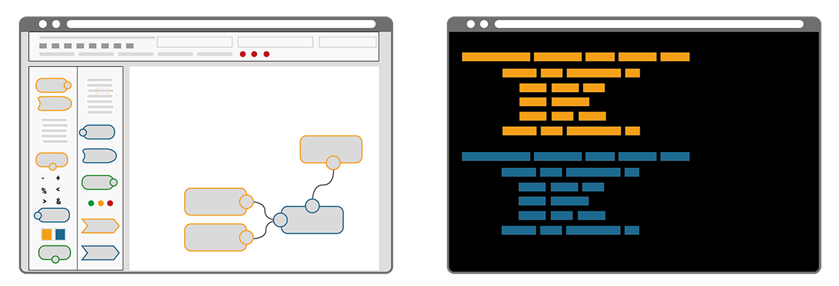
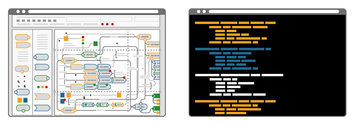
In a NC/LC based IIoT Edge Hub, all components A-G are visually represented and interrelated per drag-and-drop system on a solution design canvas. Each element is typically described via entry fields, check boxes and radio buttons in dedicated configuration windows. Immersing yourself in the code or into seemingly complex configuration files is not required. At the same time, this user convenience limits the deployment to those systems that fit into a graphical representation.
In contrast, the Infrastructure as Code (IaC) approach describes an entire infrastructure, needed for an IIoT use-case, in only one structured text file – often called the configuration or commissioning file. This file lists all of its components, called resources, and defines their specifications and interrelations in a standardized way. The commissioning file thus avoids time-consuming maneuvering of separate configurations or even scripts for each and all the different elements needed in a use-case. Everything is in one place, structured and standardized.
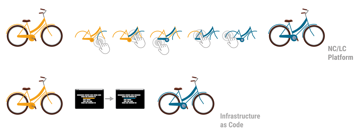
A key difference of the two approaches becomes clear by illustrating the workflow that’s required when changes are needed. Imagine a bike that consists of a number of components, each defined by its name, size, colour, function, etc. Now imagine the colour of the bike needed to be blue instead of yellow. In the IaC approach the single text-based commissioning file can be searched for “colour” and the assigned codes can be auto-replaced in a single step. Alternatively “colour” could be a resource of its own and called upon by all components, thus allowing pre-defined auto-matching colour schemes. Minimal effort, minimal risk of errors and maximum speed to deliver. In contrast, the NC/LC approach would require the administrator to click through every single bike component, select the new colour from a dropdown menu or with a radio button and confirm this selection. Obviously this route takes much longer, is prone to errors and it requires extra knowledge when colour schemes are desired.
Decision Criteria
NC/LC appears easier approachable because of its visuality. However, the problem remains in the detail of the configurations that still need to be made.
IaC on the other hand appears very technical as it resembles expert thinking in its structured approach.
Here’s how to make sense of the decision, depending on your context:
Here and there deployment or broader transformation?
When facing a single deployment, NC/LC impresses with its simple and quick handling. The drag-and-drop platform enables a fast implementation without prior knowledge and delivers quick outcomes.
But the ease of integration plays a major role in the IIoT deployment: Unlike other approaches, IaC smoothly integrates into any existing system and pipeline. There is no need to change the current infrastructure, which saves plenty of time and trouble. This also includes the potential of using different services applied on the same infrastructure – non-competitive and simultaneously. IaC also lowers the risk of flaws in processes of adaptation, as it naturally brings versioning. During the development, starting from the very first POC to the finalized environment, all steps stay traceable. Furthermore, staging deployment is easily applicable with IaC to test whether e.g. the system works properly before its final release. Additionally, a safe setup deployment can be integrated.
What’s my outlook – a limited or scaling scenario?
A crucial advantage of IaC is its limitless scalability. IaC easily adapts to every expansion, enhancement and further development. Practically, new machines or whole heterogenous shop floors are quickly connected. Also, multiple IaC can be deployed and cross-connected, if a diverse handling internally or even externally across factories is required. What makes IaC even more beneficial and suitable for scaling is its capability to design the data output individually. The commissioning files can include instructions on the frequency, format, content and critical threshold values of the data output.
In a limited use-case, NC/LC convinces with a time-saving deployment. It’s highly specialized for the specific use case, which makes it straightforward and user-friendly.
What do I expect – Static setup or continuous improvement and automation?
Thanks to its standardized deployment, IaC reduces this risk of errors and false configurations which accompanies continuous improvements. More importantly, IaC enables full automation across multiple manufacturing processes, machines, locations and even different factory operators. Besides, it permits the implementation of specific parameters, if an individual adaptation is desired.
After all, if the need occurs to change the NC/LC infrastructure to a code-based infrastructure, the conversion can become time-consuming: As users are dependent on the pre-programmed underlying code of the interface, the transition might be intransparent and produce some unexpected results. Additionally, the predefined components rule out individual specifications. This choice hampers a factories’ potential for adjustment to market changes and scalability.
Who’s working with it – anyone and their grandma or experts?
Besides the obvious aspect of user-friendliness, the security of an IIoT environment is crucial. IaC scores with a highly secure infrastructure. By using commissioning files, a closed system is created, being naturally intangible for external access. If the latter is desired, pre-defined external access can be permitted explicitly within the code. This way, the privacy protection is ensured and the access stays limited to only intended requests.
NC/LC in contrast, stands out with its user-friendliness. Reduced to a graphical interface and as little code as possible, even non-experts can set the environment up or apply changes immediately if necessary.
Conclusion
What becomes apparent is that the IaC approach is more problem generic. It can be generalized easily to other environments and conditions. NC/LC in contrast, is more problem-specific and suitable for only one precise environment.
To accelerate your decision-making and summarize the main features of both approaches, you can rely on the following rule of thumb:
- IaC: Easy things are easy and complex things are possible.
- NC/LC: Easy things are really easy but complex things may not be expressible at all.
What’s Next
For more than five years, Cybus has been relying on IaC to deploy an IIoT manufacturing environment. While realizing manifold solutions with diverse customers, our IaC solutions always contribute significantly to scalable, sustainable and efficient IIoT manufacturing environments.
If you have any questions or if you would like to get deeper into the topic of IaC, our experts are happy to provide you with further insights. You are welcome to contact us directly.
Reference
Bitkom e.V.: Paulsen, N., & Eylers, K. (2020, May 19). Industrie 4.0 – so digital sind Deutschlands Fabriken. Retrieved July 20, 2020, from https://www.bitkom.org/Presse/Presseinformation/Industrie-40-so-digital-sind-Deutschlands-Fabriken
PAC Deutschland: Vogt, Arnold (2020, April). Das Internet der Dinge im deutschen Mittelstand. Retrieved July 21, 2020, from https://iot.telekom.com/resource/blob/data/183656/e16e24c291368e1f6a75362f7f9d0fc0/das-internet-der-dinge-im-deutschen-mittelstand.pdf
Prerequisites
This lesson requires basic knowledge of
- Microservice and networking concepts
- Docker (see Docker Basics Lesson)
- MQTT (see MQTT Basics Lesson)
Introduction
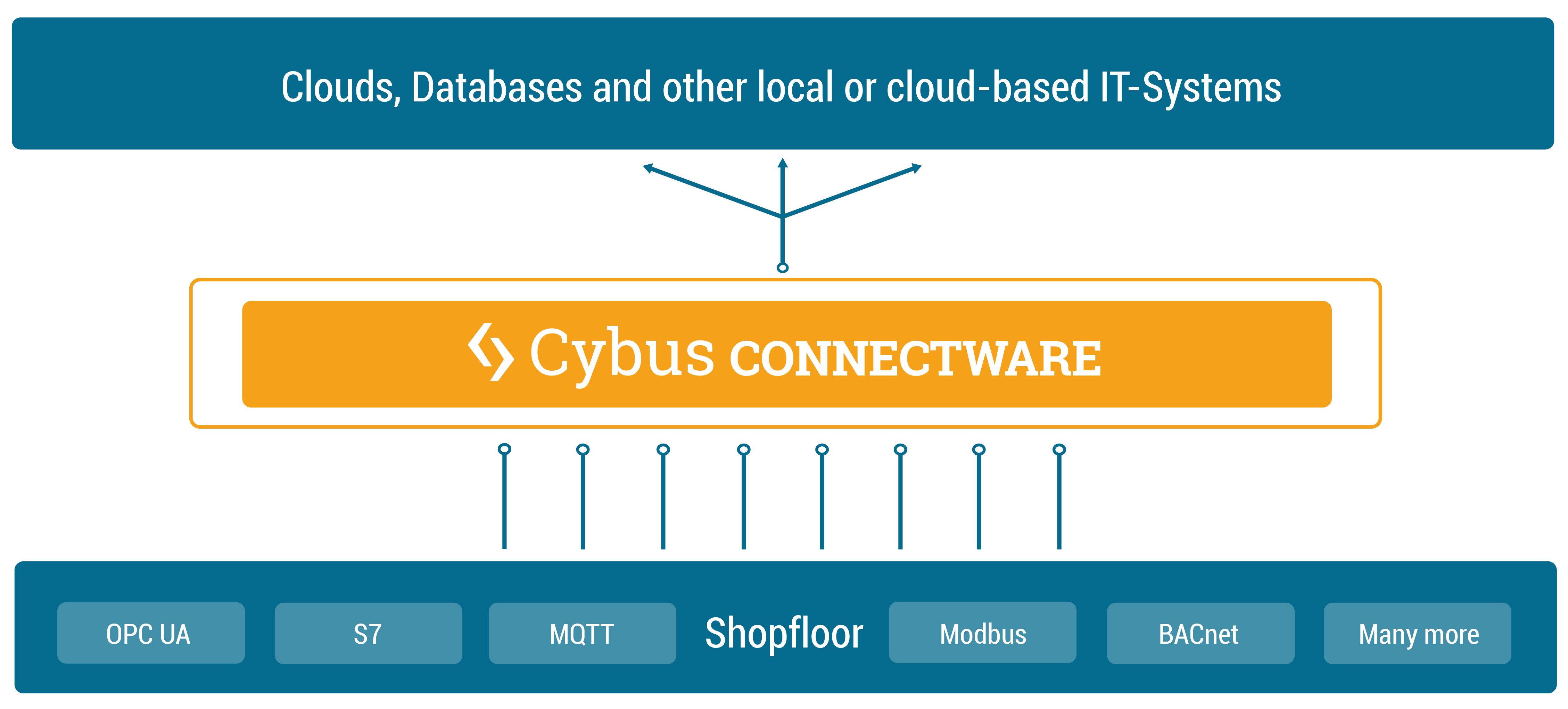
Cybus Connectware is a general and extensible on-premise data gateway that connects different devices, provides data for local systems and cloud based backends and makes data exchange transparent and secure. The components of Connectware include a data broker, protocol adapters for connectivity to standard industry protocols, a management and security layer, as well as a runtime environment to include third-party applications.
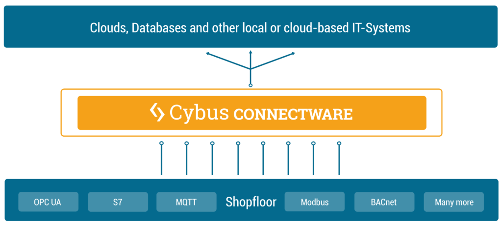
Connectware connects to the different endpoints by dedicated connectors (e.g. OPC UA, Modbus-TCP) that run as part of the Protocol Mapper in Connectware. By its microservice and API architecture Connectware supports the option of adding more connectors. And being a modern enterprise-grade IT solution based on Docker, Connectware is suitable to run on either a data centre infrastructure or standalone computers.
Connectware Overview
To begin, we’ll provide an introduction to Connectware’s architecture and its constituent parts. Connectware employs a microservice approach, with individual modules functioning in concert to establish a microservice cluster – namely, Cybus Connectware. Microservices offer numerous advantages, such as flexible scalability for individual modules or the entire application, as well as the capacity to integrate third-party applications, various databases, and even disparate programming languages into a unified application.
Connectware Architecture
In the following we will explore the Connectware architecture more closely and see what the individual microservices do and when they come into play, when we are using Connectware. We will start with a heterogene shopfloor full of data and a cloud to which we want to forward our data to – but no means of a connection between them. So the question is how are we transferring our data out of the factory, into the cloud, in a controllable, extendible and secure way?
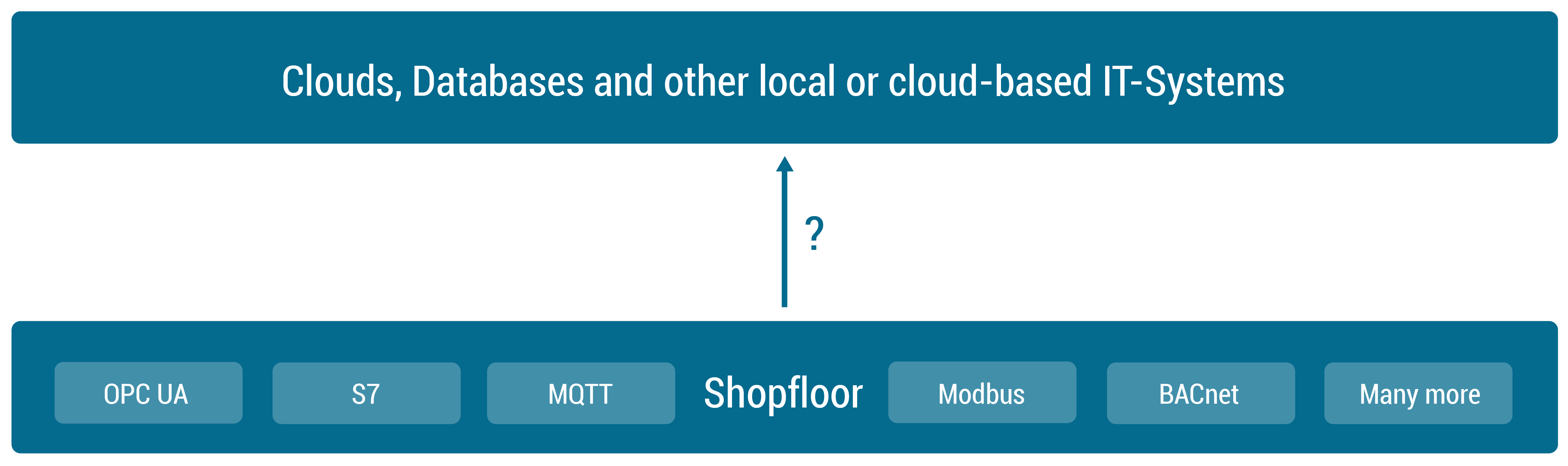
Establishing a Connection
First of all we need to start by establishing a connection between our shopfloor and the cloud application. See the following image to get an overview over the components that we will add in this section to achieve this goal.
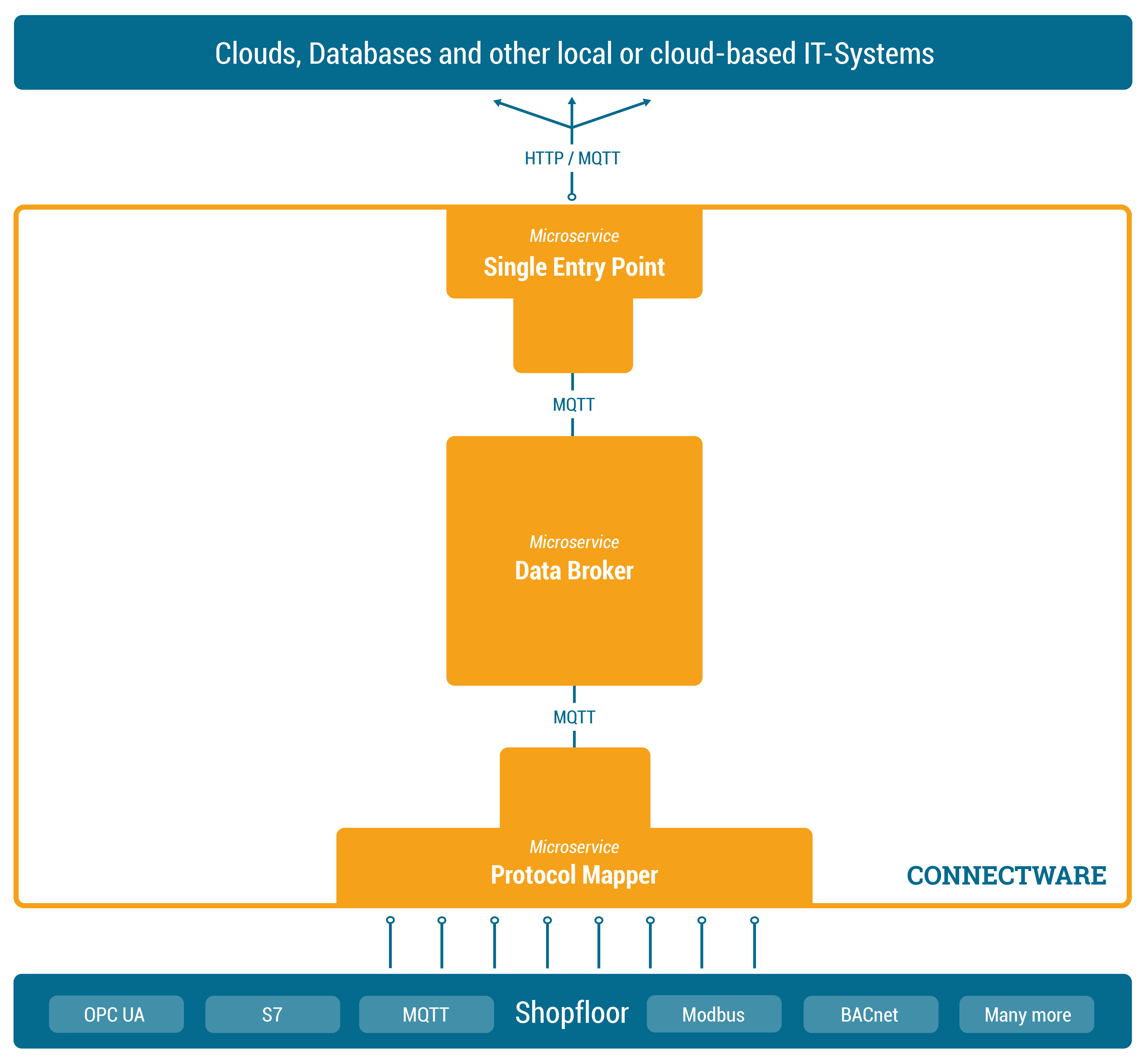
Data Broker
In order to manage and use any of our data, we need to add one central place to Connectware in which we can easily access the data – we could call it a data focal point. This single data hub gives us easy access as well as easy control over all data since all data needs to pass through this central hub. Of course this also means we need to have a Data Broker that is stable, maintainable, scalable, reliable and secure. Further we need to choose a transmission protocol that is widely used and accepted and able to handle large data flows.
The solution is to use MQTT, a standard, lightweight publish-subscribe messaging protocol on top of TCP/IP that is widely used in IoT and industrial applications. Connectware uses a high-performance MQTT broker which scales horizontally and vertically to support a high number of concurrent publishers and subscribers while maintaining low latency and fault tolerance.
So the MQTT Data Broker is the central data hub through which all data passes. Let’s now start connecting our shopfloor to the Data Broker.
Protocol Mapper
How do we get our data from different machines talking different protocols to the Connectware Data Broker? That’s where the Protocol Mapper comes into play. The Protocol Mapper uses a mapping scheme that translates various protocols to a unified MQTT/JSON API and handles the device connection management. Each device is represented by a connection resource which contains endpoints and mappings, which are used to model a MQTT topic hierarchy. All resources are defined in a text-based, human and machine readable YAML file called Commissioning File. To learn more about the configuration of connections see the How to connect to an OPC-UA server article.
Now the MQTT Data Broker is fed directly by our devices from the shopfloor via the Protocol Mapper. The next step is to forward the data to our application.
Single Entry Point
Connectware, which is running on-premise, needs to forward data to local as well as cloud applications. Therefore we need to have an access point through which Connectware can talk to the outside. Here again, it is a good practice to have one place that all the data needs to pass instead of multiple open connections that all need to be monitored. Connectware provides a Single Entry Point (or more technical Reverse Proxy) which bundles all incoming connections. Thus, to the outside the Entry Point abstracts the different microservices to one single access point. The same applies to the microservices from inside Connectware that only need to know one point to talk to when wanting to connect to the outside and forward data. Using a dedicated and high performance Reverse Proxy one can easily control all connections at this point, making a secure internet access easily possible.
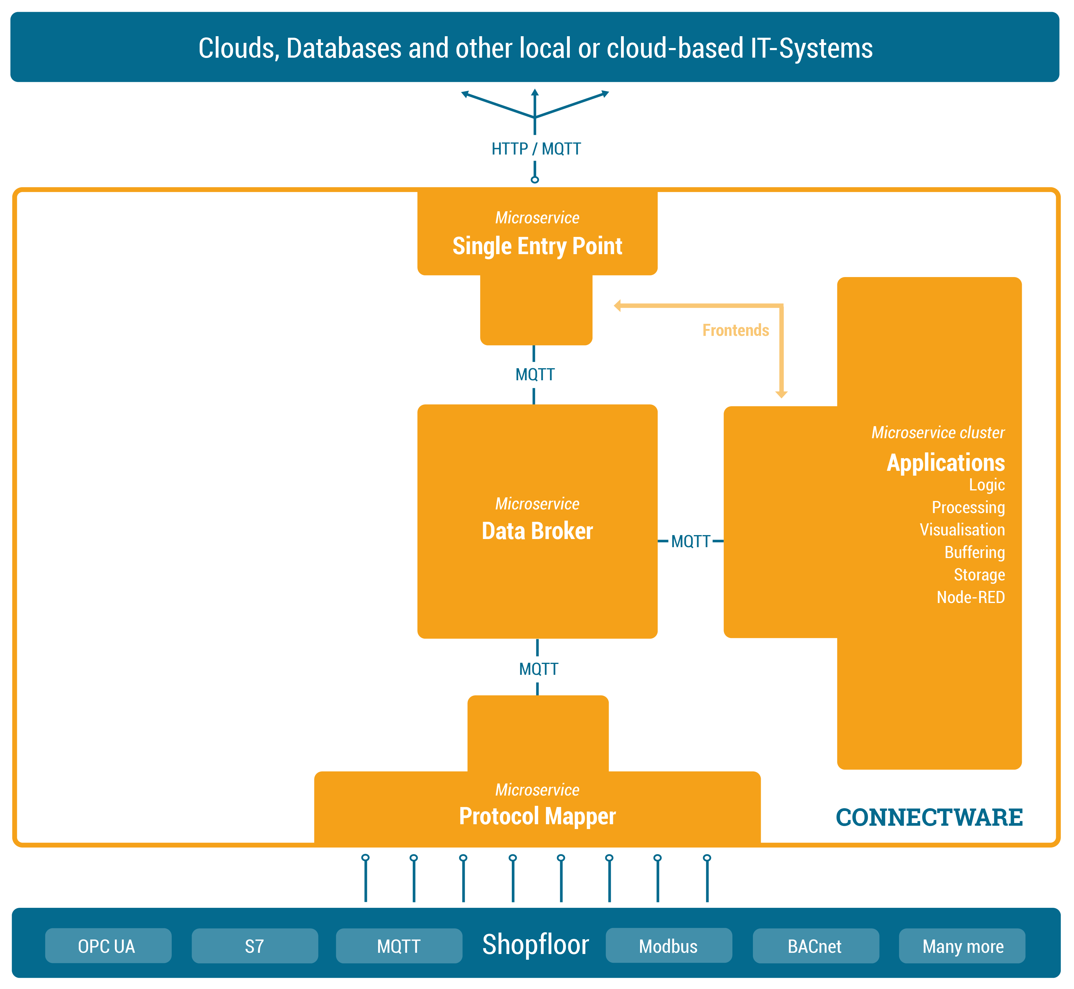
Adding Logic – The Rule Engine
At this point we are collecting data from our shopfloor and are able to forward this data to applications outside of Connectware. Connectware itself however is very well capable of applying logic to the data before forwarding it. Preprocessing the data directly on-premise and for example cutting out sensitive information, enriching data by combining data from different sources or aggregating data and send them as in one burst message to reduce costs for cloud services are just a few use-cases the Rule Engine can be used for.
What is a Service?
While Connectware allows to individually perform all settings (like managing grantees, setting permissions, starting containerized applications, etc.) the idea of Services is to bundle all these activities into a single point of configuration and execution. Services are usually built for a specific task and context. They bundle required resources with user/permission management in a easy to handle and shareable package.
How Are They Configured?
The Service configuration is done via a Commissioning File – a YAML based text file. The installation process is simply done by feeding the Commissioning File to Connectware, upon this action Connectware will review and display all the configurations that the specific Service wants to create or consume and one can decide whether or not to grant this permission to the Service (think Google Maps wants to know your location). If all permissions are agreed to then the Service will be deployed. This practice puts you in charge of your data and keeps sensitive data from leaving the factory borders.
Service Uses
Services can have a wide variety of different uses on Connectware, from data storage, preprocessing and applying logic to data on-premise prior to e.g. forwarding it to external applications. Services can also serve front-ends (visualizations, dashboards, etc) that can be used to access and control Services from the outside.
To learn more about the configuration and usage of Services see the Service Basics lesson.
Management Cluster – Making it Secure and Controllable
We are now very far in our journey of getting data out of our shopfloor. We have a Data Broker which is able to receive and forward shopfloor data and we have a runtime in which we can individually process the data. Now let’s add management and security to it.
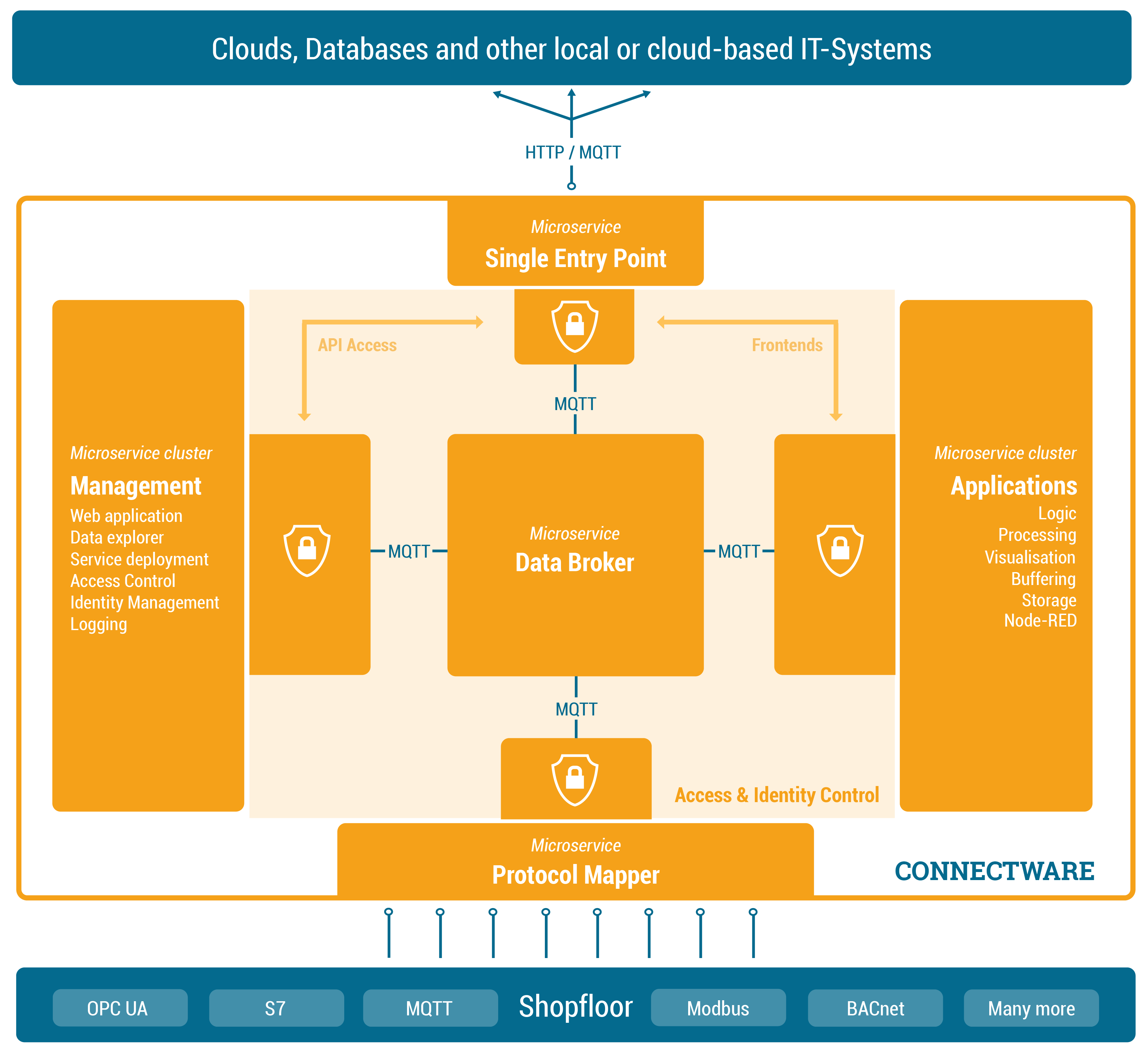
What Does the Management Cluster Do?
The Management Cluster is concerned with managing Connectware by providing the following:
- Data overview
- Supervising orchestration of resources
- Managing access control and identities
- Providing logging capabilities
How Does It Do It?
Managing Connectware is done through a modern web application through which the entire software can be configured. Here you can manage users and services through a graphical user interface. All features of the web interface can also be accessed through a REST API.
Once a client is ready to read or write data tasks like client authentication (through tokens, certificates and pre-shared passwords) and access control (who is allowed to read and write to what) are handled here. Access control is established via a simple, yet powerful control layer that handles read and write access on API endpoints and on the MQTT data broker. If required identity management can also be coupled here to directory services like Active Directory.
Connectware also has logging functionality for all system components and Service applications events. The logs can be viewed and queried via the web application. The log messages can also easily be integrated into external log management systems like ElasticSearch or Splunk.
Summary
This article covered a more technical introduction into the different microservices that build up Connectware. Starting with Connectwares scalable MQTT data broker and the Protocol Mapper which maps different industry protocol to specified MQTT topics in a standardised JSON format. Over the Rule Engine that allows complex data transformations, enriching data by combining different sources and buffering capabilities. To how we can secure and manage all of it with the Single Entry Point and the Management Cluster.
Going Further
This lesson gave overview over the basic Connectware architecture and functionality. In the following lessons we will dive way deeper into Connectware and it’s components, explaining how to connect devices, how to use and build Services yourself and how to manage Connectware. Have a look at the following articles as a starting point:
- Installing Connectware on docker-compose
- How to connect to an OPC-UA Server
Introduction
So, we want to compare two very abstract things, a classical Supervisory Control and Data Acquisition (SCADA) system against a modern Industrial Internet of Things (IIoT) system. Let’s structure the comparison by looking at the problems that each system is going to solve or in other words, the benefits that each system is intended to provide to the users.
To further structure the comparison we define the locations where the two systems are acting in:
- Things
- Gateway
- Cloud
- Mobile
The Things layer describes the location of the physical equipment the systems are going to interact with. Typically, Things on that level are not directly connected to the Internet, but typically to one or more local networks.
The Gateway describes the location where information from the Things layer is aggregated. It furthermore is the location that defines the transition between the local network(s) and the public Internet.
The Cloud layer is located in the Internet and describes a set of servers that are dealing with the data as provided by one or more Gateways.
The Mobile layer finally describes the location of a human end-user. Irrespective of the geographical location, the user will interact with the data as provided by the Cloud services always having direct access to the Internet.
You already notice that the topic is large and complex. That is why the comparison will be sliced into digestible pieces. Today’s article will start with a focus on Things and how they are represented.
Representing Things
At the lowest level we want to interact with Things, which can be – as the name suggests – quite anything. Fortunately, we are talking about IIoT and SCADA so let’s immediately reduce the scope and look at Things from an industrial perspective.
In an industrial context (especially in SCADA lingo) things are often called Devices, a general name for motors, pumps, grippers, RFID readers, cameras, sensors and so on. In other words, a Device can reflect any piece of (digitized) hardware of any complexity.
For structuring the further discussion let’s divide Devices into two kinds: actors and sensors, with actors being Devices that are „doing something“, and sensors being Devices that are „reading something“.
Having this defined, one could believe that the entire shop-floor (a company’s total set of Devices) can be categorized this way. However, this quickly turns out to be tricky as – depending on the perspective – Devices are complex entities most often including several sensors and actors at the same time.
In its extreme, already a valve is a complex Device composed of typically one actor (valve motion) and two sensors (sensing open and closed position).
View on Things
The trickiest thing for any software system is to provide interactions with Devices on any abstraction level and perspective. Depending on the user, the definition of what a Device is turns out to be completely different: the PLC programmer may see a single analog output as a Device whereas the control room operator may perceive an entire plant-subsystem as a Device (to formulate an extreme case).
Problem to Solve
Provide a system that can interact with actors and sensors at the most atomic level but at the same time provide arbitrary logical layers on top of the underlying physical realities. Those logical abstractions must fit the different end-user’s requirements regarding read-out and control and typically vary and overlap in abstraction-level (vertically) as well as in composition-level (horizontally).
Technical Solution
We will call the logical representation of a Device a Digital Twin. Digital Twins then form vertices in a tree, with the root vertex expressing the most abstract view of a Device. Lower levels of abstractions are reached by traversing the tree downwards in direction of the leaves each vertex representing a Sub-Device its parent is composed of. The leaves finally represent the lowest level of abstraction and may e.g. reflect a single physical analog input. In SCADA systems such most atomic entities are called Process Variables (PVs). The number of children per parent indicates the horizontal complexity of the respective parent. Finally the shop-floor is represented as a forest of the above described trees indicating a disjoint union of all entities.
Side Effect
In such a solution writing to or reading from a Digital Twin may result in an interaction with a physical or logical property, as Digital Twins may act on each other (as described above) or directly on physical entities.
This poses an (graph-)algorithmic challenge of correctly identifying all Digital Twins affected by a failure or complete loss of connection to a physical property and for the entire access control layer that must give different users different permissions on the available properties.
SCADA vs IIoT
SCADA systems have a very strong focus on creating logical representations of Devices at a very early stage. A full set of a logical Device hierarchy is established and visualized to the user already on-premise. Most of the data hence never hit the cloud (i.e. the Internet) but is used to immediately feedback into the system or to the operator. Although distributed, SCADA systems aggregate data within (private) local networks and hence have less focus on Internet security or web-standards for communication.
IIoT systems, in contrast, try to make no assumptions on where the representation from raw information to logical Devices is happening. Furthermore, they do not assume that data is used solely for observing and controlling a plant but for completely – yet unknown – use cases, such as integration into other administrative layers of an enterprise. Consequently, communication is prepared to follow most recent standards of security and transport protocols from the beginning on and much effort is undertaken to have a very flexible, albeit semantically clear description of the raw Device data to be consumed by any other higher abstraction layer.
Final Words
Hopefully, you could already grasp some fundamental differences between the two systems. In the following articles we will sharpen these differences and have a look at further locations of activity (Gateway, Cloud and Mobile).
In a final article we will demonstrate how Cybus Connectware implements all the discussed requirements for a modern IIoT system and how you can use it for your special use-case.
Introduction
This article covers Docker, including the following topics:
- Installing Docker
- Raising containers from the command line
- Managing containers and reading log output
- Using Dockerfiles
- Scouting docker hub for fun and profit
Prerequisites
What is Docker
Maybe this sounds familiar. You have been assigned a task in which you had to deploy a complex software onto an existing infrastructure. As you know there are a lot of variables to this which might be out of your control; the operating system, pre-existing dependencies, probably even interfering software. Even if the environment is perfect at the moment of the deployment what happens after you are done? Living systems constantly change. New software is introduced while old and outdated software and libraries are getting removed. Parts of the system that you rely on today might be gone tomorrow.
This is where virtualization comes in. It used to be best practice to create isolated virtual computer systems, so called virtual machines (VMs), which simulate independent systems with their own operating systems and libraries. Using these VMs you can run any kind of software in a separated and clean environment without the fear of collisions with other parts of the system. You can emulate the exact hardware you need, install the OS you want and include all the software you are dependent on at just the right version. It offers great flexibility.
It also means that these VMs are very resource demanding on your host system. The hardware has to be powerful enough to create virtual hardware for your virtual systems. They also have to be created and installed for every virtual system that you are using. Even though they might run on the same host, sharing resources between them is just as inconvenient as with real machines.
Introducing the container approach and one of their main competitors, Docker. Simply put, Docker enables you to isolate your software into containers (Check the picture below). The only thing you need is a running instance of Docker on your host system. Even better: All the necessary resources like OS and libraries cannot only be deployed with your software, they can even be shared between individual instances of your containers running on the same system! This is a big improvement above regular VMs. Sounds too good to be true?
Well, even though Docker comes with everything you need, it is still up to you to assure consistency and reproducibility of your own containers. In the following article, I will slowly introduce you to Docker and give you the basic knowledge necessary to be part of the containerized world.
Getting Docker
Before we can start creating containers we first have to get Docker running on our system. Docker is available for Linux, Mac and just recently for Windows 10. Just choose the version that is right for you and come back right here once you are done:
Please notice that the official documentation contains instructions for multiple Linux distributions, so just choose the one that fits your needs.
Even though the workflow is very similar for all platforms, the rest of the article will assume that you are running an Unix environment. Commands and scripts can vary when you are running on Windows 10.
Your First Docker Container
Got Docker installed and ready to go? Great! Let’s get our hands on creating the first container. Most tutorials will start off by running the tried and true „Hello World“ example but chances are you already did it when you were installing Docker.
So let’s start something from scratch! Open your shell and type the following:
  docker run -p 8080:80 httpd
Code-Sprache: YAML (yaml)
If everything went well, you will get a response like this:
  Unable to find image 'httpd:latest' locally
  latest: Pulling from library/httpd
  f17d81b4b692: Pull complete
  06fe09255c64: Pull complete
  0baf8127507d: Pull complete
  07b9730387a3: Pull complete
  6dbdee9d6fa5: Pull complete
  Digest: sha256:90b34f4370518872de4ac1af696a90d982fe99b0f30c9be994964f49a6e2f421
  Status: Downloaded newer image for httpd:latest
  AH00558: httpd: Could not reliably determine the server's fully qualified domain name, using 172.17.0.2. Set the 'ServerName' directive globally to suppress this message
  AH00558: httpd: Could not reliably determine the server's fully qualified domain name, using 172.17.0.2. Set the 'ServerName' directive globally to suppress this message
  [Mon Nov 12 09:15:49.813100 2018] [mpm_event:notice] [pid 1:tid 140244084212928] AH00489: Apache/2.4.37 (Unix) configured -- resuming normal operations
  [Mon Nov 12 09:15:49.813536 2018] [core:notice] [pid 1:tid 140244084212928] AH00094: Command line: 'httpd -D FOREGROUND'
Code-Sprache: YAML (yaml)
Now there is a lot to go through but first open a browser and head over to: localhost:8080
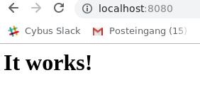
What we just achieved is, we set up and started a simple http server locally on port 8080 within less than 25 typed characters. But what did we write exactly? Let’s analyze the command a bit closer:
docker– This states that we want to use the Docker command line interface (CLI).run– The first actual command. It states that we want to run a command in a new container.-p 8080:80– The publish flag. Here we declare what Docker internal port (our container) we want to publish to the host (the pc you are sitting at). the first number declares the port on the host (8080) and the second the port on the Docker container (80).httpd– The image we want to use. This contains the actual server logic and all dependencies.
IMAGES
Okay, so what is an image and where does it come from? Quick answer: An image is a template that contains instructions for creating a container. Images can be hosted locally or online. Our httpd image was hosted on the Docker Hub. We will talk more about the official docker registry in the Exploring the Docker Hub part of this lesson.
HELP
The Docker CLI contains a thorough manual. So whenever you want more details about a certain command just add --help behind the command and you will get the man page regarding the command.
Now that we understand what we did we can take a look at the output.
  Unable to find image 'httpd:latest' locally
  latest: Pulling from library/httpd
  f17d81b4b692: Pull complete
  06fe09255c64: Pull complete
  0baf8127507d: Pull complete
  07b9730387a3: Pull complete
  6dbdee9d6fa5: Pull complete
  Digest: sha256:90b34f4370518872de4ac1af696a90d982fe99b0f30c9be994964f49a6e2f421
  Status: Downloaded newer image for httpd:latest
Code-Sprache: YAML (yaml)
The httpd image we used was not found locally so Docker automatically downloaded the image and all dependencies for us. It also provides us with a digest for our just created container. This string starting with sha256 can be very useful for us! Imagine that you create software that is based upon a certain image. By binding the image to this digest you make sure that you are always pulling and using the same version of the container and thus ensuring reproducibility and improving stability of your software.
While the rest of the output is internal output from our small webserver, you might have noticed that the command prompt did not return to input once the container started. This is because we are currently running the container in the forefront. All output that our container generates will be visible in our shell window while we are running it. You can try this by reloading the webpage of our web server. Once the connection is reestablished, the container should log something similar to this:
172.17.0.1 - - [12/Apr/2023:12:25:08 +0000] "GET / HTTP/1.1" 200 45
Code-Sprache: YAML (yaml)
You might have also noticed that the ip address is not the one from your local machine. This is because Docker creates containers in their own Docker network. Explaining Docker networks is out of scope for this tutorial so I will just redirect you to the official documentation about Docker networks for the time being.
For now, stop the container and return to the command prompt by pressing ctrl+c while the shell window is in focus.
Managing Docker Containers
Detaching Docker Containers
Now that we know how to run a container it is clear that having them run in an active window isn’t always practical. Let’s start the container again but this time we will add a few things to the command:
  docker run --name serverInBackground -d -p 8080:80 httpd
Code-Sprache: YAML (yaml)
When you run the command you will notice two things: First the command will execute way faster then the first time. This is because the image that we are using was already downloaded the last time and is currently hosted locally on our machine. Second, there is no output anymore besides a strange string of characters. This string is the ID of our container. It can be used to refer to its running instance.
So what are those two new flags?
--name– This is a simple one. It attaches a human readable name to our container instance. While the container ID is nice to work with on a deeper level, attaching an actual name to it makes it easier to distinguish between running containers for us as human beings. Just keep in mind that IDs are unique and your attached name might not!-d– This stands fordetachand makes our container run in the background. It also provides us with the container ID.
Sharing resources: If you want to you can execute the above command with different names and ports as many times as you wish. While you can have multiple containers running httpd they will all be sharing the same image. No need to download or copy what you already have on your host.
Listing Docker Containers
So now that we started our container, make sure that it is actually running. Last time we opened our browser and accessed the webpage hosted on the server. This time let’s take another approach. Type the following in the command prompt:
  docker ps
Code-Sprache: YAML (yaml)
The output should look something like this:
  CONTAINER ID    IMAGE    COMMAND              CREATED             STATUS           PORTS                  NAMES
  018acb9dbbbd    httpd    "httpd-foreground"   11 minutes ago      Up 11 minutes    0.0.0.0:8080->80/tcp   serverInBackground
Code-Sprache: YAML (yaml)ps– The ps command prints all running container instances including information about ID, image, ports and even name. The output can be filtered by adding flags to the command. To learn more just typedocker ps --help.
Inspecting Docker Containers
Another important ability is to get low level information about the configuration of a certain container. You can get these information by typing:
  docker inspect serverInBackground
Code-Sprache: YAML (yaml)
Notice that it does not matter if you use the attached name or the container ID. Both will give you the same result.
The output of this command is huge and includes everything from information about the image itself to network configuration.
Note: You can execute the same command using an image ID to inspect the template configuration of the image.
To learn more about inspecting docker containers please refer to the official documentation.
Crawling Inside the Docker Container
We can even go in deeper and interact with the internals of the container. Say we want to try changes to our running container without having to shut it down and restart it every time. So how do we approach this?
Like a lot of Docker images, httpd is based upon a Linux image itself. In this case httpd is running a slim version of Debian in the background. So being a Linux system, we can access a shell inside the container. This gives us a working environment that we are already familiar with. Let’s jump in and try it:
  docker exec -it -u 0 serverInBackground bash
Code-Sprache: YAML (yaml)
There are a few new things to talk about:
exec– This allows us to execute a command inside a running container.-it– These are actually two flags.-i -twould have the same result. While i stands for interactive (we need it to be interactive if we want to use the shell) t stands for TTY and creates a pseudo version of the Teletype Terminal. A simple text based terminal.-u 0– This flag specifies the UID of the user we want to log in as. 0 opens the connection as root user.serverInBackground– The container name (or ID) that we want the command to run in.bash– At the end we define what we actually want to run in the container. In our case this is the bash environment. Notice that bash is installed in this image. This might not always be the case! To be safe you can addshinstead ofbash. This will default back to a very stripped down shell environment by default.
When you execute the command you will see a new shell inside the container. Try moving around in the container and use commands you are familiar with. You will notice that you are missing a lot of capabilities. This has to be expected on a distribution that is supposed to be as small as possible. Thankfully httpd includes the apt packaging manager so you can expand the capabilities. When you are done, You can exit the shell again by typing exit.
Getting Log Output
Sometimes something inside your containers just won’t work and you can’t find out why by blindly stepping through your configuration. This is where the Docker logs come in.
To see logs from a running container just type this:
  docker logs serverInBackground -f --tail 10
Code-Sprache: YAML (yaml)
Once again there are is a new command and a few new flags for us:
logs– This command fetches the logs printed by a specific container.-f– Follow the log output. This is very handy for debugging. With this flag you get a real time update of the container logs while they happen.--tail– Chances are your container is running for days if not months. Printing all the logs is rarely necessary if not even bad practice. By using thetailflag you can specify the amount of lines to be printed from the bottom of the file.
You can quit the log session by pressing ctrl+c while the shell is in focus.
Stopping a Detached Docker Container
If you have to shut down a running container the most graceful way is to stop it. The command is pretty straight forward:
  docker stop serverInBackground
Code-Sprache: YAML (yaml)
This will try to shutdown the container and kill it, if it is not responding. Keep in mind that the stopped container is not gone! You can restart the container by simply writing:
  docker start serverInBackground
Code-Sprache: YAML (yaml)
Killing the Docker Container – A Last Resort
Sometimes if something went really wrong, your only choice is to take down a container as quickly as possible.
  docker kill serverInBackground
Code-Sprache: YAML (yaml)
Note: Even though this will get the job done, killing a container might lead to unwanted side effects due to not shutting it down correctly.
Removing a Container
As we already mentioned, stopping a container does not remove it. To show that a stopped container is still managed in the background just type the following:
  docker container ls -a
Code-Sprache: YAML (yaml)container– This accesses the container interaction.ls– Outputs a list of containers according to the filters supplied.-a– Outputs all containers, even those not running.
CONTAINER ID    IMAGE    COMMAND              CREATED              STATUS                      PORTS    NAMES
ee437314785f    httpd    "httpd-foreground"   About a minute ago   Exited (0) 8 seconds ago             serverInBackground
Code-Sprache: YAML (yaml)
As you can see even though we stopped the container it is still there. To get rid of it we have to remove it.
Just run this command:
  docker rm serverInBackground
Code-Sprache: YAML (yaml)
When you now run docker container ls -a again you will notice that the container tagged serverInBackground is gone. Keep in mind that this only removes the stopped container! The image you used to create the container will still be there.
Removing the Image
The time might come when you do not need a certain image anymore. You can remove an image the same way you remove a container. To get the ID of the image you want to remove you can run the docker image ls command from earlier. Once you know what you want to remove type the following command:
  docker rmi <IMAGE-ID>
Code-Sprache: YAML (yaml)
This will remove the image if it is not needed anymore by running docker instances.
Exploring the Docker Hub
You might have asked yourself where this mysterious httpd image comes from or how I know which Linux distro it is based on. Every image you use has to be hosted somewhere. This can either be done locally on your machine or a dedicated repository in your company or even online through a hosting service. The official Docker Hub is one of those repositories. Head over to the Docker Hub and take a moment to browse the site. When creating your own containers it is always a good idea not to reinvent the wheel. There are thousands of images out there spreading from small web servers (like our httpd image) to full fledged operating systems ready at your disposal. Just type a keyword in the search field at the top of the page (web server for example) and take a stroll through the offers available or just check out the httpd repo. Most of these images hosted here offer help regarding dependencies or installation. Some of them even include information about something called a Dockerfile..
Writing a Dockerfile
While creating containers from the command line is pretty straight forward, there are certain situations in which you do not want to configure these containers by hand. Luckily enough we have another option, the Dockerfile. If you have already taken a look at the example files provided for httpd you might have an idea about what you can expect.
So go ahead and create a new file called ‚Dockerfile‘ (mind the capitalization). We will add some content to this file:
FROM httpd:2.4
COPY ./html/ /usr/local/apache2/htdocs/
Code-Sprache: YAML (yaml)
This is a very barebone Dockerfile. It basically just says two things:
FROM– Use the provided image with the specified version for this container.COPY– Copy the content from the first path on the host machine to the second path in the container.
So what the Dockerfile currently says is: Use the image known as httpd in version 2.4, copy all the files from the sub folder ‚./html‘ to ‚/usr/local/apache2/htdocs/‘ and create a new image containing all my changes.
For extra credit: Remember the digest from before? You can use the digest to pin our new image to the httpd image version we used in the beginning. The syntax for this is:
FROM <IMAGENAME>@<DIGEST-STRING>
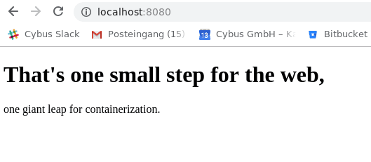
Code-Sprache: YAML (yaml)Now, it would be nice to have something that can actually be copied over. Create a folder called html and create a small index.html file in there. If you don’t feel like writing one on your own just use mine:
<!DOCTYPE html>
<html>
  <body>
    <h1>That's one small step for the web,</h1>
    <p>one giant leap for containerization.</p>
  </body>
</html>
Code-Sprache: YAML (yaml)
Open a shell window in the exact location where you placed your Dockerfile and html folder and type the following command:
  docker build . -t my-new-server-image
Code-Sprache: YAML (yaml)build– The command for building images from Dockerfiles.– Thebuildcommand expects a path as second parameter. The dot refers to the current location of the shell prompt.-t– The tag flag sets a name for the image that it can be referred by.
The shell output should look like this:
  Sending build context to Docker daemon  3.584kB
  Step 1/2 : FROM httpd:2.4
  ---> 55a118e2a010
  Step 2/2 : COPY ./html/ /usr/local/apache2/htdocs/
  ---> Using cache
  ---> 867a4993670a
  Successfully built 867a4993670a
  Successfully tagged my-new-server-image:latest
Code-Sprache: YAML (yaml)
You can make sure that your newly created image is hosted on your local machine by running
  docker image ls
Code-Sprache: YAML (yaml)
This will show you all images hosted on your machine.
We can finally run our modified httpd image by simply typing:
  docker run --name myModifiedServer -d -p 8080:80 my-new-server-image
Code-Sprache: YAML (yaml)
This command should look familiar by now. The only thing we changed is that we are not using the httpd image anymore. Instead we are referring to our newly created ‚my-new-server-image‘.
Let’s see if everything is working by opening the Server in a browser.
Summary
By the time you reach these lines you should be able to create, monitor and remove containers from pre-existing images as well as create new ones using Dockerfiles. You should also have a basic understanding of how to inspect and debug running containers.
Where to Go from Here
As was to be expected from a basic lesson there is still a lot to cover. A good place to start is the Docker documentation itself. Another topic we didn’t even touch is Docker Compose, which provides an elegant way to orchestrate groups of containers.
Learn More
Introduction
This article will be covering Wireshark including the following topics:
- Getting Wireshark
- Software overview
- Basic filtering
- Example usage
What is Wireshark
Wireshark is a network packet analyzer. It is used to capture data from a network and display its content. Being an analyzer, Wireshark can only be used to measure data but not manipulate or send it. Wireshark is open source and free which makes it one of the most popular network analyzer available.
Getting Wireshark
Wireshark is available for Linux, Windows and Mac through the official website. For more information about building Wireshark from source please take a look at the official developers guide.
Running Wireshark
Depending on your operating system and user settings you might have to run Wireshark with admin privileges to capture packets on your network. If your welcome screen is blank and does not show any network interfaces it usually means that your user account is lacking the necessary access rights.
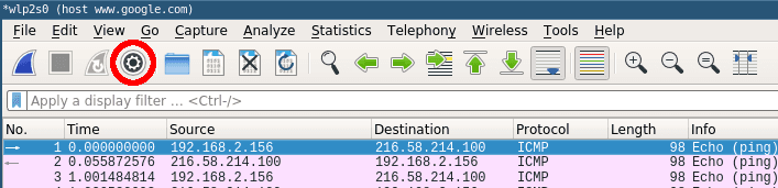
Your First Capture
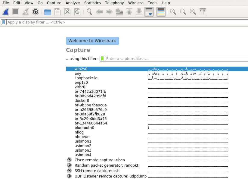
Once Wireshark is started you will be greeted by a welcome screen like the one shown above listing all available network connections. A small traffic preview is shown next to the interface names so it is easy to distinguish between interfaces with or without direct network access. To finally start capturing data on your network you first have to select one or more of these network interfaces by simply clicking on them. To select multiple interfaces at once just hold down ctrl and select all interfaces you want to listen on. Once selected you can start recording packets by clicking the start icon in the top left of the user interface.
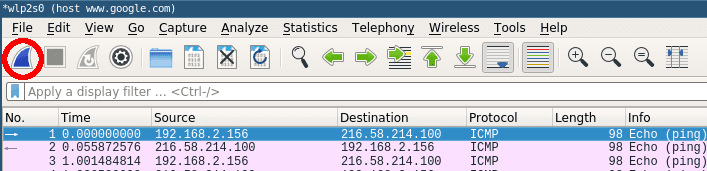
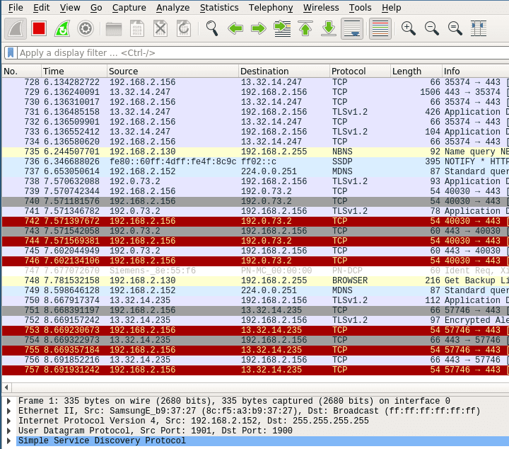
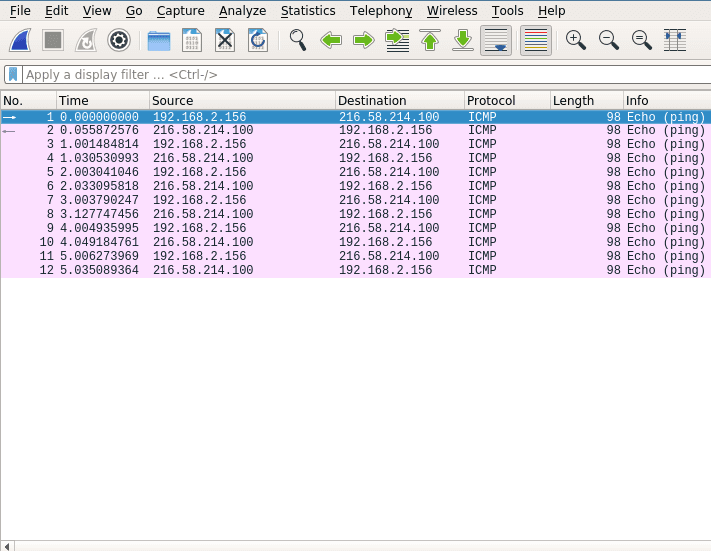
The window will change to the main capturing view and immediately display everything passing the network on your selected capturing device as see below.
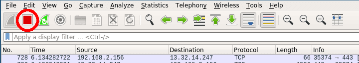
Stop the current capturing process by clicking on the red stop button.
Filtering Traffic
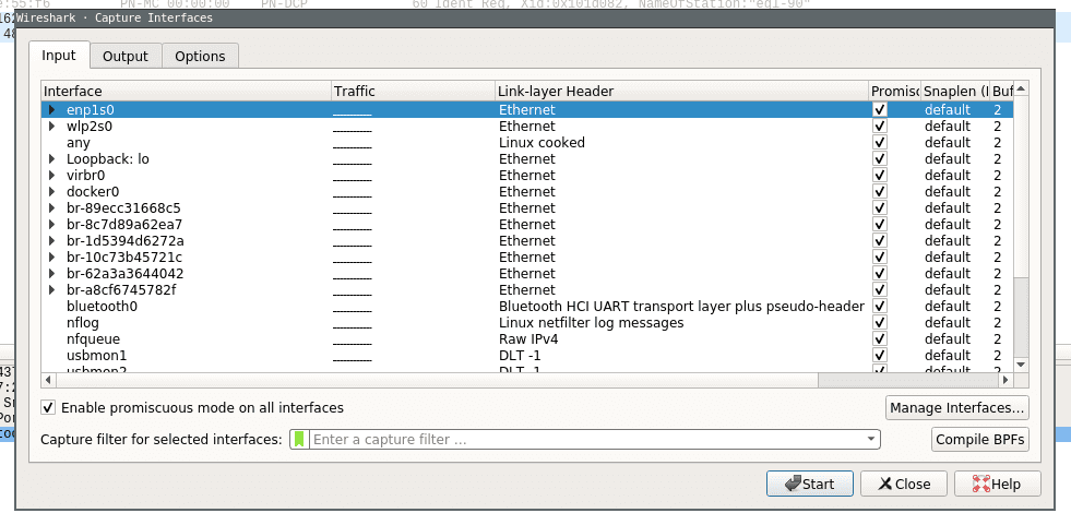
Even the smallest network will produce a lot of static data that can result in very large capture files. To avoid slowdowns you should not capture unfiltered network traffic. To do so open the capture configuration window by clicking on the cogwheel icon.
This will open the capture configuration menu. This menu provides options similar to those you already saw on the welcome screen. You can select network devices, set capture filters and configure the capturing process. This time we want to apply a filter before we start capturing data. Select the network interface of your choice and just type ‚tcp‘ into the capture filter dialog box on the bottom of the configuration window like below.
Now when you now start capturing again only packets applicable to the tcp protocol filter are captured and displayed.
More on Filters
Wireshark provides a powerful filter language which not only allows you to narrow down the packets you want to capture but also to sort, follow or even compare their content. This section will only scratch the surface of what is possible with Wireshark so for the time being please consult the Wireshark Wiki for further information about creating filters.
It is a common mistake to believe that capture filters and display filters work the same way in Wireshark. While capture filters change the outcome of the capturing process, display filters can be applied to already running capturing processes to narrow down what to display. Furthermore they use different filter language syntax.
Capture Filter Example
To narrow down our captured data to only include packets from a certain ip range:
src net 192.168.2.0/24Code-Sprache: YAML (yaml)Display Filter Example
The same can be done to filter the already captured data in the main window:
ip.addr == 192.168.2.0/24Code-Sprache: YAML (yaml)Combining Filters
To find exactly what you are looking for on your network you can concatenate different filters. If you want to capture packets from a certain host and port you can simply add both filters together:
host 192.168.2.100 and port 20Code-Sprache: YAML (yaml)You can specify data that you want to explicitly exclude:
host www.google.com and not (port 20 or port 80)Code-Sprache: YAML (yaml)This would only capture data from a certain host which is not transferred on port 20 or 80.
Collecting Data
A standard example to see actual network traffic is to ping a host and collect the data.
Just run a capture and set the capture filter to the host you are going to ping (www.google.com would be a popular choice).
host www.google.comGo ahead and start the capturing process. Without any connections to your host open the main window should stay empty for now.
Next open a terminal window and ping the host you specified in the capture filter. Within a few moments you should see the first packets.
Once you have captured some packets press the stop button.
Analyzing at the Data
After collecting data the user interface contains three main parts. Those being the packet list pane, the packet details pane and packet bytes pane.
On top is the packet list pane. This view displays a summary of all the captured packets. You can choose any of the packets by just selecting and the other two views will adapt to the selection. Go ahead and select any of the packets and notice how the other two views change.
The one in the middle is the packet details pane. It shows more details about the packets you select in the packet list pane.
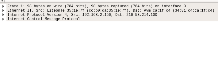
On the bottom the packet bytes pane displays the actual data transferred in the packets.
Using these sections you can view the traffic and break it down for analysis.
Summary
Wireshark is a powerful network packet analyzer. It offers everything you need to capture, filter and view your local network traffic. After reading through this article you should have all the basic knowledge necessary to create and filter simple captures.
Learn More
Prerequisites
- Basic knowledge of networking concepts
- Basic protocol understanding.
Introduction
This article will be covering the MQTT Protocol including:
- What is MQTT?
- Where does MQTT come from?
- Client and Broker
- Protocol Concepts
- MQTT Topics
- MQTT QOS
- Retained messages in MQTT
What is MQTT?
MQTT or Message Queuing Telemetry Transport is a lightweight publish (send a message) subscribe (wait for a message) protocol. It was designed to be used on networks that have low-bandwidth, high-latency and could be unreliable. Since it was designed with these constraints in mind, it’s perfect to send data between devices and is very common in the IoT world.
Where Does MQTT Come From?
MQTT was invented by Dr Andy Stanford-Clark of IBM, and Arlen Nipper of Arcom (now Eurotech), in 1999. They invented the protocol while working on the SCADA system for an oil and gas company that needed to deliver real time data. For 10 years, IBM used the protocol internally. Then, in 2010 they released MQTT 3.1 as a free version for public use. Since then many companies have used the protocol including Cybus.
If you’re interested in learning more you can click here to read the transcript of an IBM podcast where the creators discuss the history and use of MQTT.
Client and Broker in MQTT
Client
A client is defined as any device from a microcontroller to a server as long as it runs a MQTT client library and connects to a MQTT broker over a network. You will find that many small devices that need to connect over the network use MQTT and you will find that there are a huge number of programming languages that support MQTT as well.
Find a list of libraries here.
Broker
The broker is defined as the connector of all clients that publish and receive data. It manages active connections, filtering of messages, receiving messages and then routing messages to the correct clients. Optionally, it can also handle the authentication and authorization of clients.
Find a list of brokers here.
For information on how they work together continue on to the next section.
MQTT Protocol Concepts
MQTT uses the publish (send a message) subscribe (wait for a message) pattern. This is an alternative approach to how a normal client (asks for data) server (send back data) pattern works. In the client server pattern, a client will connect directly to a component for requesting data and then immediately receive a response back. In the publish subscribe pattern, the connection between the components is handled by a third party component called a broker.
All messages go through the broker and it handles dispatching the correct message to correct receivers. It does that through the use of a topic. A topic is a simple string that can have hierarchical levels separated by ‚/‘.
Examples Topics:
- house/toaster/temp
- house/washer/on
- house/fridge/on
The MQTT client can listen for a message by subscribing to a specific topic. It will then receive data when a MQTT client publishes a message on that topic.
Example
Client A:                                 Broker
subscribe /house/toaster/temp  ---------->  |
                                            |
                                            |                       Toaster Device:
                                            | <-------- publish /house/toaster/temp
                                            |
                                            |
Client A   < ------ Receive Message ------  |Code-Sprache: YAML (yaml)
This publish subscribe pattern offers a couple of advantages:
- Publisher and subscriber do not need to know anything about one another because the broker handles the receiving and sending of messages.
- There can be a time difference between the clients that are sending information to one another since the protocol is event based.
- The subscriber and publisher can process the information at different times which means they don’t block each other from sending or receiving new information.
Topics in MQTT
Topics are the way that data is organized in MQTT. They are structured in a hierarchy manner using the ‚/‘ as a separator. It’s very similar to how folders and files are structured in a file system. A few things to remember about topics are that they are case sensitive, must use UTF-8 and have to have at least 1 character.
Example of Basic Topics
- /
- house
- house/toaster
- house/toaster/temp
Multiple Subscriptions
A client can also subscribe to multiple topics at once using wildcards. The 2 wildcards in MQTT are:
- # (multi level): replaces many topics and must be set at the end of hierarchy.
- + (single level): replaces one topic.
The level being the level of the topic hierarchy tree that you want to subscribe to.
Example Multi Level
Subscribe to house/#
- house/temp
- house/toaster/temp
- house/tv/on
The ‘#’ wildcard gets all the information under the topic ‘house’.
Example Single Level
Subscribe to house/+/light
- house/frontroom/light
- house/bedroom/light
- house/porch/light
NOT
- house/frontroom/temp
- house/bedroom/lamp
The ‘+’ wildcard gets all the topics that has ‘light’ as a keyword.
Publishing MQTT Topics
An MQTT client can only publish to an individual topic. Meaning you cannot use wildcards.
$SYS Topics
The only topics you will find in a broker after start is the $SYS topics. These topics are usually reserved for publishing internal statistics about the broker such as the number of current client connections.
If you would like to read more specifics on the requirements of topics see the MQTT specification.
MQTT QOS
QOS (Quality of Service) is defined as the agreement between the broker and the client that deals with the guarantee that a message was delivered. MQTT defines 3 levels of QOS.
QOS 0 (At Most Once)
This is the fastest QOS level(works as “fire and forget”). When a message is sent across the network no reply from the broker is sent acknowledging that it received the message. The sending message is then deleted from the client sending queue so no repeat messages will be sent.
QOS 1 (At Least Once)
This level is the default mode of transfer. The message is guaranteed to be delivered at least once. It will continue to send the message with a DUP flag until an acknowledgment message is sent. This could result in duplicate messages being sent.
QOS 2 (Exactly Once)
This is the slowest level as it requires 4 messages. The message is always delivered exactly once.
- The sender sends the message and waits for a response from the broker.
- The sender receives the response from the broker. If it doesn’t it sends the request again with a DUP flag.
- The sender sends a message saying that it received the response and awaits acknowledgment.
- The sender receives acknowledgment and deletes the message. If not it sends another message saying that it received the response with a DUP flag.
Retained Messages in MQTT
Normally when a client publishes a message to the broker, the broker will delete the message after routing to the correct subscribing clients. But what if a client subscribes to a topic after the message is sent? Then it will receive no data until another message is published. This could be desirable in certain situations but in other situations you may want the client to have the last published data. This is the purpose of the retain flag. If set to true when a message is sent the broker will cache the message and route it to any new subscribing clients. There is only 1 retained message per topic and if a new message is published it will replace the retained message.
Summary
MQTT is a lightweight publish subscribe protocol. It is defined with a broker client relationship and organizes its data in hierarchy structures called topics. When publishing messages you can specify a QOS level which will guarantee that a message is sent and specify a retain level for a message so a subscribing client can receive retained data after connecting.